A First Look at Some Atlanta Housing Data

I recently found out that the Federal Housing Authority publishes a ton of granular housing data and wanted to start exploring the data for Atlanta, where I live. I’m not sure there will be anything revelatory in here, but sometimes it’s fun to look at a map.

FHA Public Use Data

The PUDB single-family datasets include loan-level records that include data elements on the income, race, and gender of each borrower as well as the census tract location of the property, loan-to-value (LTV) ratio, age of mortgage note, and affordability of the mortgage. New for 2018 are the inclusion of the borrower’s debt-to-income (DTI) ratio and detailed LTV ratio data at the census tract level.

I was stunned when I read that this is a loan-level dataset. That means we can see every loan that is sold to Freddie Mac and Fannie Mae along with the census tract it was located in. I have always wanted to explore location-based models and this seems like a great dataset to play around with.

For those less interested in the technical details I’ll quickly show some plots I found interesting, and then once all the normal people have left I’ll go deep into the models I used to smooth the data and put the maps together.

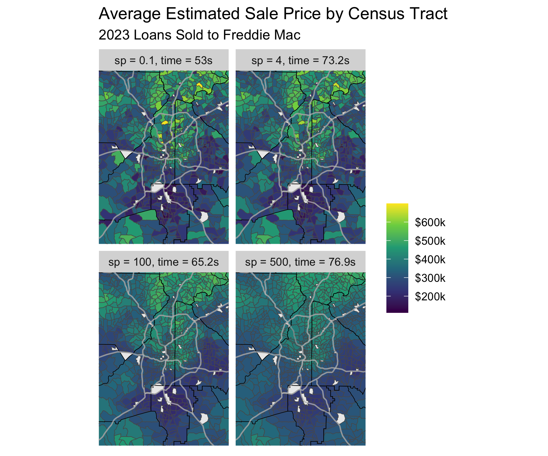
The first plot we’ll discuss is the Average Sale Price by Census Tract for homes sold in 2023:

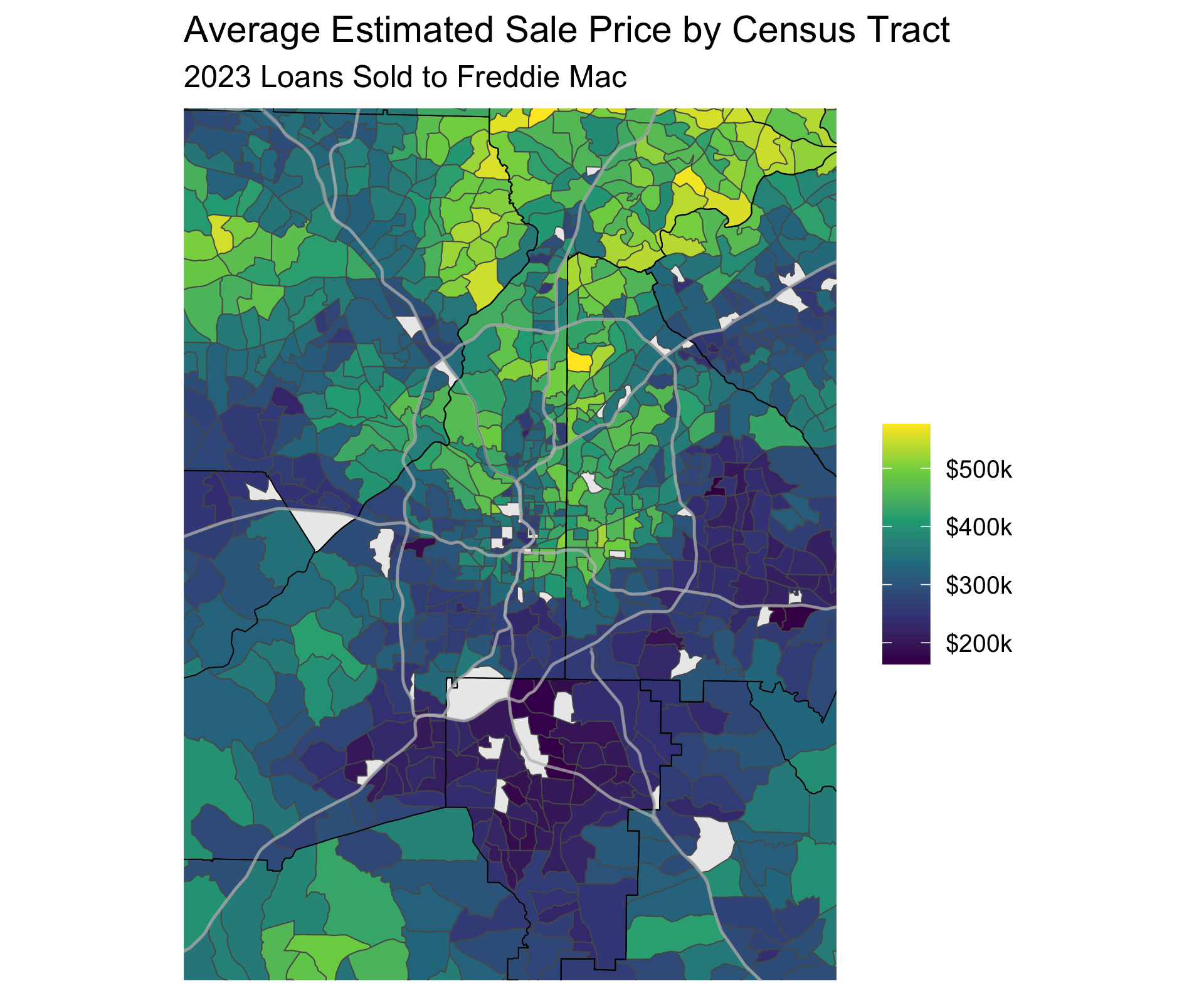
I’ll take this opportunity to note that this is only looking at single-family homes that were sold to Freddie Mac (I only looked at the Freddie Mac file, but my understanding is there shouldn’t be a bias in which loans get sold to Freddie Mac vs Fannie Mae) in 2023. I smoothed the estimates so that the map was a little easier to digest. The smoothing was done by shrinking the difference in home prices between neighboring census tracts, so essentially each tract’s value in the map is a blend of their actual average sale price and all their neighbor’s average sale price. If you want to read more scroll to the technical details section.

Home Sales

We can see the parts of Atlanta that have the most sales in this plot (this plot is not smoothed):

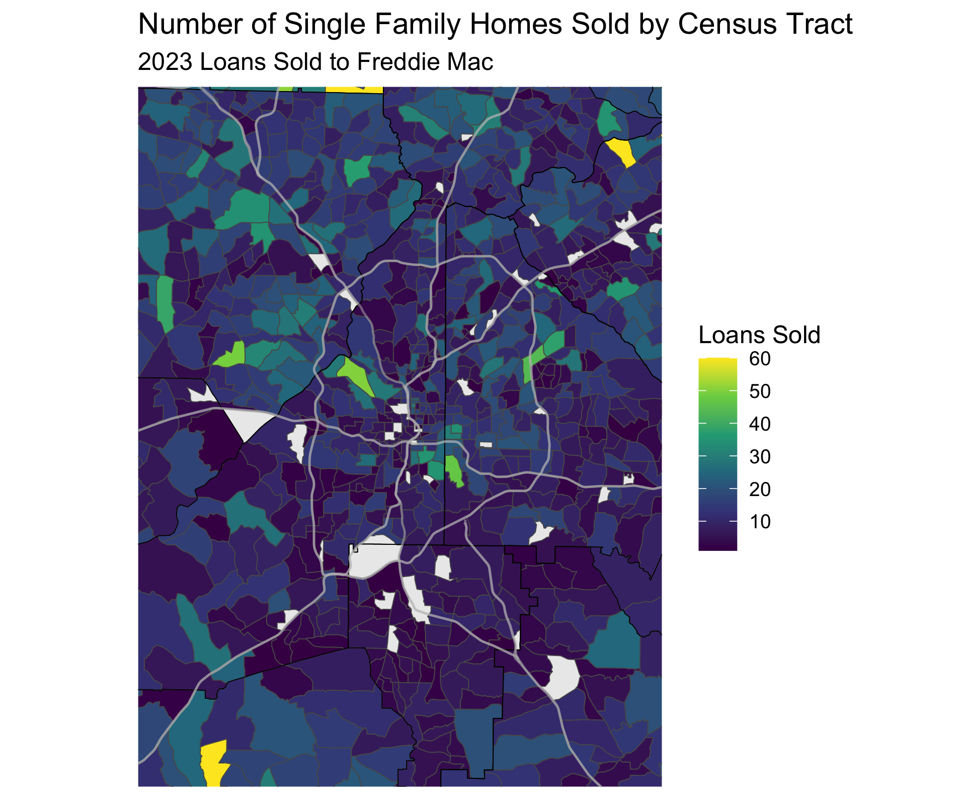
The bright yellow Census Track in the NE corner, on the border of Fulton and Gwinnett County, is or is near Duluth. I wonder if there was a new subdivision that finished in 2023 to explain the number of mortgages sold? Seems like a strange result otherwise.

First Time Buyers

In addition to Home Values I think one of the most interesting trends we can track over time is where people can buy their first home around Atlanta. Because of restrictive Land Use policies we are simply running out of homes close to the city that are affordable. I plan to look at previous years of Housing data to see how these locations have changed over time.

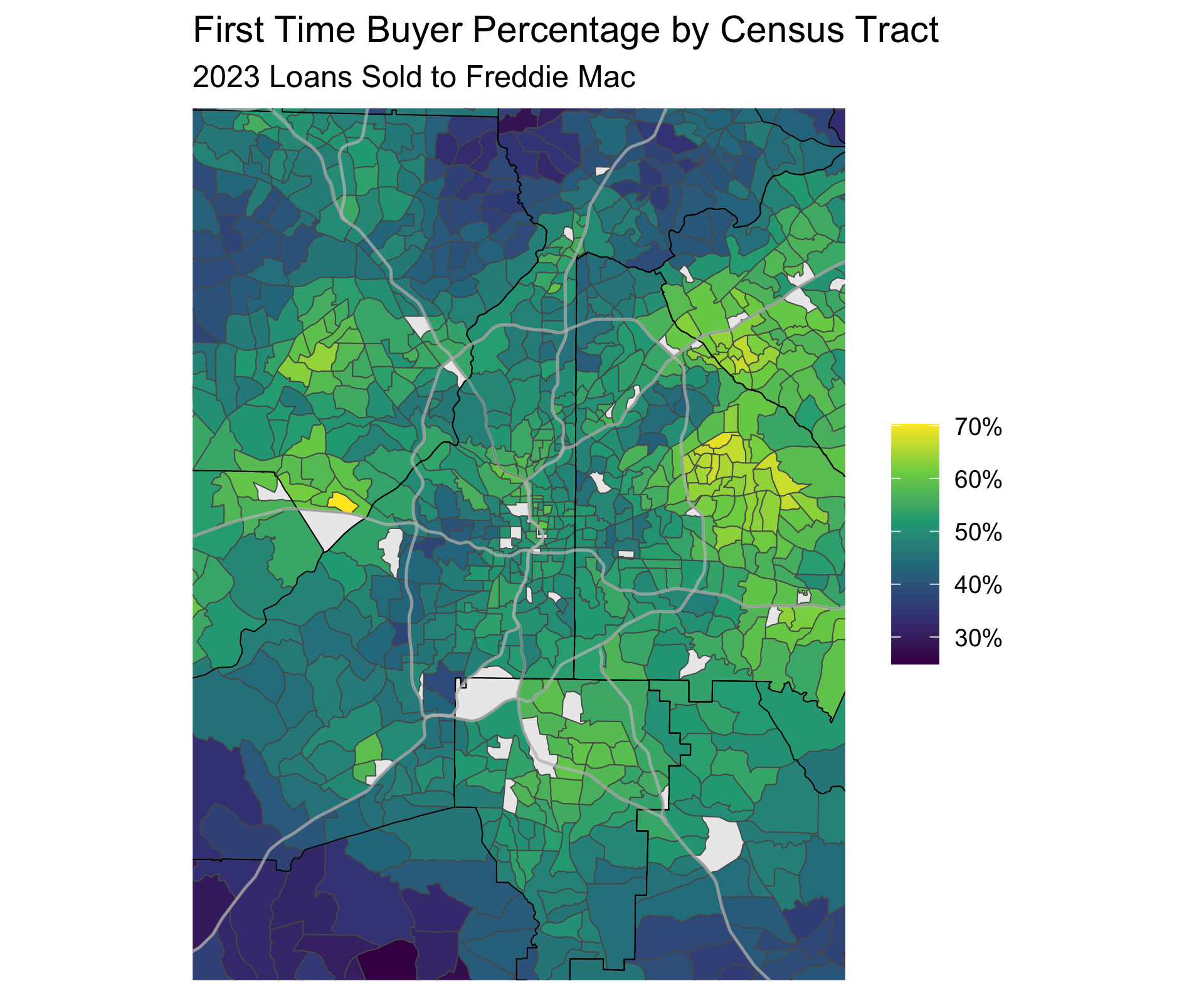
You can see how the Census Tracts with the highest rate of first time buyers are OTP (if you know you know). You can also see the more expensive suburbs that are out of reach for most first time home buyers. I want to explore the trends between home prices and home sales in the ITP census tracts that should have more condos and townhomes, but also some really expensive homes, so see if we can parse out the dual trends there. But that will have to wait for a future post.

This is it for now, but I’m excited to explore the dataset in more detail. What else should I be looking at?

Technical details

In this section I’ll discuss how we smoothed the data. Smoothing is straight-forward, especially with the incredible sf, spdep, and mgcv packages, but requires some potentially complicated data transformations. The basic idea of smoothing location data is that neighboring locations (in our case census tracts) should have similar values. As you get further away then we should be less confident that two census tracts would have similar values. We can do this using a Gaussian Markov Random Field (GMRF).

But you might be asking yourself why is this smoothing step necessary? Well, for one I think it makes prettier charts. But more importantly it can help us deal the small and varying number of home sales within each district. On average each census tract only has 11.8 home sales. While the average home price is an accurate metric for, well, the average home price in a census tract, statistical theory tells us that we can calculate a more accurate estimate of the actual average home price by decreasing the variance using a smoothed estimate. Using a smoothed estimate will cause a census tract that has a much higher average home price than it’s neighbors to be shrunk towards it’s neighbor’s estimates. If that census tract has a lot of home sales it will be shrunk less than if it only has a few home sales. These estimates should be better predictors of the real but unobserved values.

Markov Random Fields

Like I said earlier the smoothing is performed by fitting a GMRF model. If each location $j$ has a value of a quantity of interest $\gamma_j$ and we want a smooth estimate of that value $J(\gamma_j)$ we can penalize the difference between the district’s value and the value of all it’s neighbors (expressed as a function $nei(j)$ which tells us the indices for the regions neighboring our region of interest)

[ J(\gamma) = \sum_j^m \sum_{i \in nei(j)} (\gamma_i - \gamma_j)^2 ]

We can capture the neighboring districts as a matrix where a value of -1 tells us that district $i$ is neighbors with district $j$, the diagonal is the count of neighbors for each district $j$, and all other values are 0. We can see how this plays out with an example. If we have 4 districts our neighbor penalty matrix may look like:

\begin{array}{cc} \begin{bmatrix} 1 & 0 & -1 & 0 \\ 0 & 2 & -1 & -1 \\ -1 & -1 & 2 & 0 \\ 0 & -1 & 0 & 1 \end{bmatrix} & \begin{bmatrix} \gamma_1 \\ \gamma_2 \\ \gamma_3 \\ \gamma_4 \end{bmatrix} \end{array}

If you write out the equations for the 2nd district you get

[ 2\gamma_2 - \gamma_3 - \gamma_4 = (\gamma_2 - \gamma_3) + (\gamma_2 - \gamma_4) ]

So the penalty we add to our loss function when we estimate our value for district two is the sum ( (technically the squared sum, just not in this toy example) of the difference between it’s estimate and it’s two neighbors.

That’s kind of it. We just need our list of neighbors and mgcv will create this neighbor matrix and fit the model. Each census tract will be assigned a parameter the model will fit a model balancing the error of our estimates with the squared difference between neighboring districts. If you want an example check out the code directly on github.

Low Rank Smoothers

There is actually an additional way to smooth our estimates. The prior smoothing using an MRF will reduce the difference between neighboring districts, but will still estimate a parameter for each district. This can take a long time, especially if you have 937 census tracts to estimate! We can speed things up using a low-rank smoother. Essentially we transform our penalty matrix to one in which the penalties are a function of an eigenvalue matrix with the eigen-values on the diagonal. By penalizing this matrix we set some eigenvalues to 0 and thus we increase the number of non-zero parameters. I’m going to devote a full post to this subject because 1.) it fascinates me that its possible and 2.) I don’t really understand how it works. So follow me @statmills on X or BlueSky to get notified of any future posts.

Smooth Examples

To show the effect that the size of the low rank dimension has on our model lets show the difference between 4 basis dimensions values.

fit_smooth_lr = function(df, output = 'avg_home_value', k = 100, xt = xt, sp=NULL){
  model_formula = as.formula(glue("{output} ~ s(census_tract_fct, bs='mrf', xt=xt, k={k})"))
  time1 = Sys.time()
  model = gam(model_formula,
              data=df, method='REML',
              weights=df$num_loans,
              sp=sp)
  model_preds = df[c("geometry", "CountyCode", "CensusTractCode")]
  model_preds[glue('{output}_pred')] = fitted(model)
  model_preds$k = if_else(k < 0, 'None', as.character(k))
  model_preds$sp = sp
  time2 = Sys.time()
  model_preds$time = as.numeric(time2 - time1, units = 'secs')
  return(model_preds)
}

home_value_k_preds = map_dfr(c(10, 100, 500, -1), 
                             ~ fit_smooth_lr(ct_first_time_map, k = .x))

The model call tells us that we are fitting a smooth as a function of our census tracts (s(census_tract_fct,) using a Markov Random Field basis (bs='mrf') with a list of neighbors xt and a basis dimension of k. We fit each model, extract the predictions, record the time it took, and return the results.

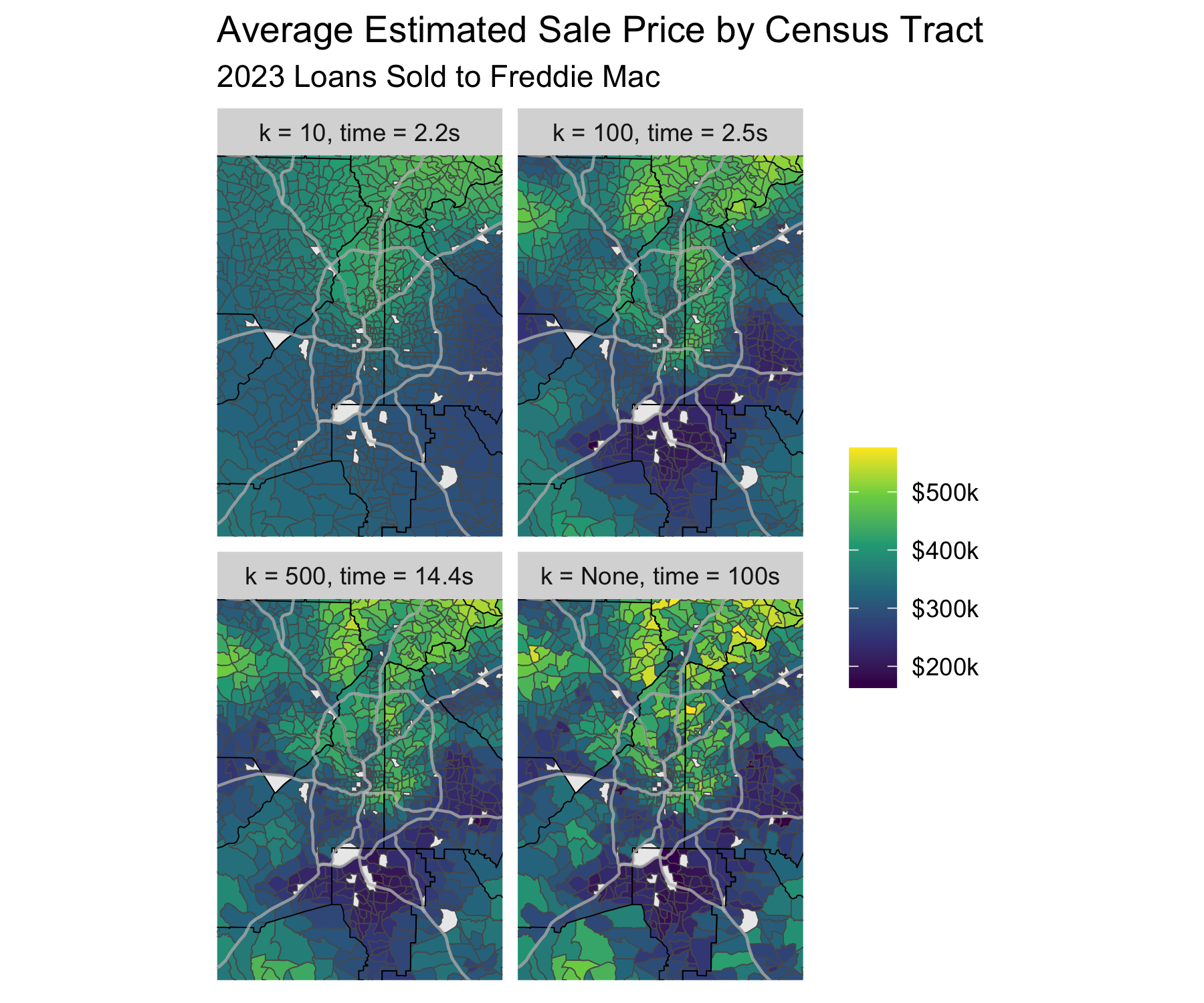
The difference in predictions between using a basis with 500 dimensions and a full-rank basis is not that different, but the low-rank model fits more than 5x faster.

We could accomplish similar smoothing with a larger penalty (mgcv automatically picks one for us using Restricted Maximum Likelihood, see the method arg). However, we would still fit a coefficient for each census tract and not enjoy any speedups.

I think that’s it for now! I hope to conduct more analysis using this dataset, especially looking at changes over the years.

Sources

Debugging Sources: LLMs help a lot, but often you still need a stackoverflow deep dive to solve problems. I want to shout the random blog posts out that helped me debug some errors I encountered while writing this post: