Let’s say you have a trend you are trying to model that you know to be monotonically increasing or decreasing; this could be something like default as a function of risk, power usage as a function of temperature, or CO2 emissions over time. Generalized Additive Models (GAMs) are a great general purpose modeling tool that you could use to model these relationships, but they are unconstrained and could have undesired shape behavior. It turns out that there are variations of GAMs that allow for enforcing a constraint on a spline curve; Penalized splines (P-splines) and Shape Constrained P-Splines (SCOP). This contraint could be an always increasing or decreasing function, or even a convex or concave shape. P-splines use a penalty matrix to enfore the constraint by penalizing differences between neighboring coefficients that violate the desired trend. SCOPs, and sometimes the more general term Shape Constrained Additive Models (SCAM), use a different parameterization of a GAM that I wanted to learn more about. This blog post is an attempt to recreate the logic in the SCAM paper using python and JAX. If you want to use these types of models for real there is an R-package for SCAMs and a P-spline implementation in python using the pygam library.
Shape Constrained What-now?
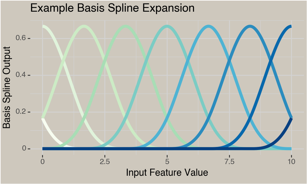
Shape Constrained Additive Models :) SCAMs use a reparameterization of a traditional B-spline basis to enforce a constraint. If you want a refresher on B-Splines and GAMs I wrote an introductory focused post last year. Briefly though B-Splines are a basis expansion consisting of individual basis splines (B-Spline) that cover the range of the data. A GAM is usually expressed as a B-spline with coefficients for each basis that are learned from the data while estimating some trend.
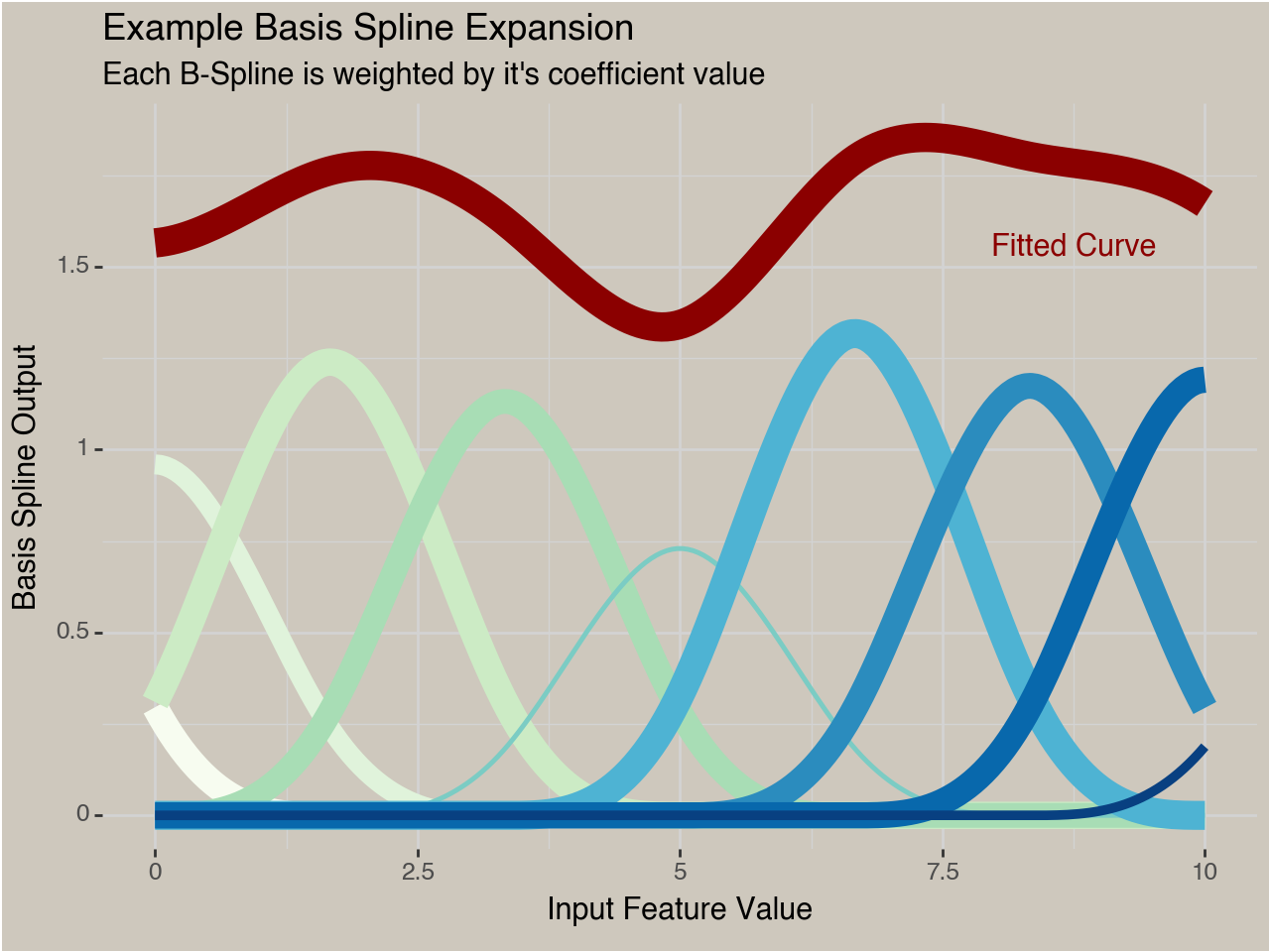
When we add learned coefficients for each spline we are fitting a model $\hat{Y} = \mathbf{X}\mathbf{\beta}$ :
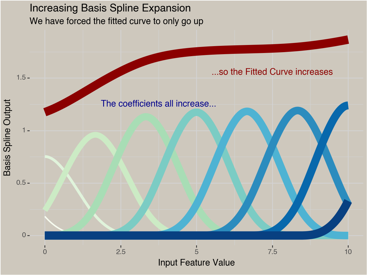
With a reparameterization we can model trends with a specific shape, for example a monotonically increasing function.
How do we do this reparameterization? A traditional B-spline can be expressed as
[ \hat{Y} = \mathbf{X}\mathbf{\beta} ]
Where $\mathbf{X}$ is the $n$ by $j$ spline-transformed data matrix and $\mathbf{\beta}$ are the $j$ coefficients found from fitting a model to the data. If we don’t impose any constraints or penalties this could just be fit as a standard GLM. But now we want to force the curve to either always go up, or always go down.
This new expression of the B-spline basis has two components:
- A transformation on the coefficients of a traditional B-spline to ensure they are always positive
- A constraint matrix inserted in the $\mathbf{X} \mathbf{\beta}$ multiplication.
The first step of the reparameterization is simple enough, we apply the exponential function to our unconstrained coefficients:
[ \tilde{\beta} = \exp(\beta) ]
Now each transformed coefficient is stricly positive. We’ll see the reason for this below.
The constraint matrix combines these transformed coefficients so that the desired constraint is adhered to. We’ll walk through how this works for a decreasing trend. We know our transformed coefficients are strictly positive. So if we want our curve to always decrease, then each successive coefficient we multiply with our $X$ matrix needs to be strictly smaller than the previous coefficient. We can accomplish this by applying another reparameterization to our coefficients. Lets set the first coefficient in our new coefficient vector $\overline{\beta}$ as our first stricly positive coefficient:
[ \overline{\beta_1} = \tilde{\beta_1} ]
The next coefficient now needs to be less than this first value. One way to do that is to subtract our $\tilde{\beta_2}$ value from $\tilde{\beta_1}$ and use the result as the 2nd transformed coefficient. Since we know $\tilde{\beta_2}$ is positive (from using the exponential function) then we know that $\beta_1$ is strictly larger than $\tilde{\beta_1} - \tilde{\beta_2}$. We can repeat this logic the whole way down our vector of coefficients:
\begin{align} \overline{\beta_1} &= \tilde{\beta_1} \\ \overline{\beta_2} &= \tilde{\beta_1} - \tilde{\beta_2} \\ \overline{\beta_3} &= \tilde{\beta_1} - \tilde{\beta_2} - \tilde{\beta_3} \\ \dots \end{align}We don’t have to write these equations out by hand, we can leverage a lower triangle matrix where all values are negative 1 except the first column.
\begin{array}{cc} \mathbf{\overline{\beta}} = \begin{bmatrix} 1 & 0 & 0 & 0 \\ 1 & -1 & 0 & 0 \\ 1 & -1 & -1 & 0 \\ 1 & -1 & -1 & -1 \\ \end{bmatrix} \mathbf{\tilde{\beta}} \end{array}The SCAM paper doesn’t create this 2nd intermediate coefficient vector $\mathbf{\overline{\beta}}$ but instead just includes the constraint matrix $\mathbf{Sigma}$ in the prediction matrix multiplication:
[ \hat{Y} = \mathbf{X} \mathbf{\Sigma} \mathbf{\tilde{\beta}} ]
To summarize the process we first start with unconstrained coefficients that we transform into positive numbers. Then we combine them in a way so that the resulting coefficients on each input column in $\mathbf{X}$ are decreasing as we move along the coefficients. Then we multiply those values by the basis matrix to generate our predictions.
Different constraint matrices result in different shapes; you can view the constraint matrices for convex, concave, and many other shapes in the SCAM paper.
Comparison with P-splines
P-splines enforce a monotonic constraint using a penalty matrix instead of a constraint matrix. This penalty matrix uses the difference matrix to punish any difference between neighboring coefficients that goes against this desired trend.
\begin{bmatrix} -1 & 1 & 0 & 0 \\ 0 & -1 & 1 & 0 \\ 0 & 0 & -1 & 1 \\ \end{bmatrix}For decreasing trends only positive values for $\beta_{i+1} - \beta_i$ would contribute a penalty to the loss function, while a negative value would not contribute anything. If I have time for another post I’ll do a more thorough comparison to see how the differences actually manifest in model fitting between the two methods.
An Example: Japanese Cherry Blossom Data
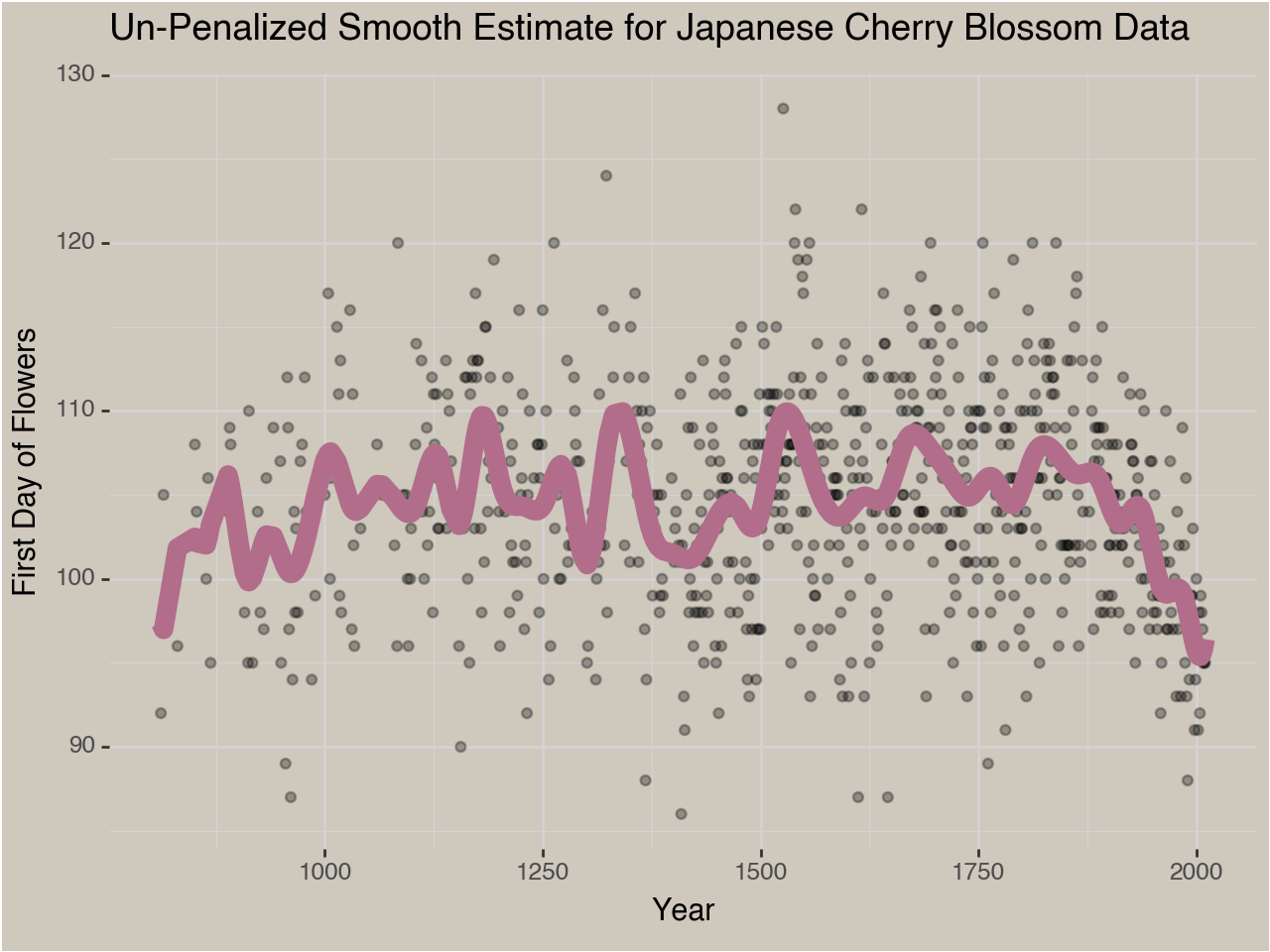
There is a phenomenal dataset of the first day of the Cherry Blossoms blooming in the Japanese Royal Gardens every year since 812 AD. I want to estimate the long-term trend of this date moving up over time due to Global Warming. There are natural, short-term fluctuations in this data based on the local climate in Japan so an accurate model of the year to year fluctuations will not be monotonically decreasing. For this post I’m only interested in the long-term trend which I’m going to assume only goes one way. We’ll read in some data and build our model. I’m only going to show some code cells and output, but if you want to see the full code it is available on my github.
flower_df = pl.read_csv(FLOWER_DATA, truncate_ragged_lines=True)
flower_df.columns = ['year', 'flower_doy', 'flower_date', 'source', 'ref']
flower_df_clean = flower_df.filter(pl.col('flower_doy').is_not_null())
print(flower_df_clean.head().to_pandas().to_markdown(index=False))
  year    flower_doy     flower_date     source ref   -------- ------------- --------------- ---------- ------------------------
   812            92             401          1 NIHON-KOKI

   815           105             415          1 NIHON-KOKI

   831            96             406          1 NIHON-KOKI

   851           108             418          1 MONTOKUTENNO-JITSUROKU

   853           104             414          1 MONTOKUTENNO-JITSUROKU   --------------------------------------------------------------------------
# calc splines
yearly_spline = SplineTransformer(n_knots = 50, include_bias = True).fit_transform(flower_df_clean[['year']])
#yearly_spline = np.concat([np.ones((yearly_spline.shape[0], 1)),yearly_spline], axis=1)
flower_df_clean = flower_df_clean.with_columns(flower_moy = flower_df_clean['flower_doy'] / 30)
DV = 'flower_moy'
base_model = GeneralizedLinearRegressor(fit_intercept=False).fit(X=yearly_spline, y=flower_df_clean[DV])
flower_df_clean = flower_df_clean.with_columns(base_preds = base_model.predict(yearly_spline))
def generate_constraint_matrix(coefs, direction='dec'):
    '''Generate a constraint matrix for a monotonic function.

    I was debugging for a while so I did this super inneficiently to make sure I was doing it right
    '''
    con = np.zeros((len(coefs), len(coefs)))

    if direction=='inc':
        for i in range(len(coefs)):
            for j in range(len(coefs)):
                if i >= j:
                    con[i, j] = 1
    if direction=='dec':
        for i in range(len(coefs)):
            for j in range(len(coefs)):
                if i >= j:
                    con[i, j] = -1

        con[:, 0] = 1

    return con

cons_matrix = generate_constraint_matrix(base_model.coef_)
cons_matrix[:5, :5]
array([[ 1.,  0.,  0.,  0.,  0.],
       [ 1., -1.,  0.,  0.,  0.],
       [ 1., -1., -1.,  0.,  0.],
       [ 1., -1., -1., -1.,  0.],
       [ 1., -1., -1., -1., -1.]])
def apply_shape_constraint(coef_b, direction='dec'):
    """
    Applies shape constraints to the coefficient vector, excluding the intercept.
    coef_b: shape-constrained coefficients (excluding intercept).
    direction: 'inc' for increasing, 'dec' for decreasing.
    """
    beta_exp = jnp.exp(coef_b)  # Ensure monotonicity
    cumulative_sums = jnp.array(generate_constraint_matrix(coef_b, direction))
    constrained_coefs = jnp.matmul(cumulative_sums, beta_exp.T)
    return constrained_coefs

test_coefs = np.random.uniform(size=5)
mono_coefs = apply_shape_constraint(test_coefs)
print(f'Latent Coefficients: {np.round(test_coefs, 2)}\n')
print(f'Constrained Coefficients: {np.round(mono_coefs, 2)}')
Latent Coefficients: [0.81 0.08 0.37 0.3 0.17]
Constrained Coefficients: [2.24 1.16 -0.29 -1.64 -2.83]
Fitting a Model with JAX
Previously I used the excellent glum package to fit a GAM using a
penalty matrix. We can’t use that approach for SCAMs though because the
constraint is enforced as we get predictions at the model matrix level,
not as an additional penalty in the loss function. So we need a way to
learn the optimal coefficients directly. I thought this would be a great
chance to use JAX. JAX is a “numpy + autodif” library in python that
many advanced Deep Learning models are built with these days. The reason
we would use JAX to fit our model is that JAX will calculate a
derivative of a function automatically. So all we need to do is write a
loss function that accepts our input parameters, the unconstrained
coefficients, and JAX will automatically calculate 1st and 2nd order
gradients that we can pass to scipy’s optimization function minimize.
I’ll write a helper function to get the predictions and then write
functions to calculate our loss function, gradients, and hessians. I do
want to re-iterate again that our loss function and it’s derivatives
operate on the unconstrained parameter values before we exponentiate
them. Then we (well really scipy) apply the necessary transformations at
each run after applying the necessary gradient updates to the raw
paramter values.
def predict_mono_bspline(coefs, X=yearly_spline, direction='dec'):
    """
    Predicts values from a monotonic B-spline model without an intercept.
    coefs: full coefficient vector
    X: basis spline matrix.
    direction: 'inc' for increasing, 'dec' for decreasing.
    """
    coef_b = coefs  # Shape-constrained coefficients

    # Apply the shape constraint only to coef_b
    constrained_coefs = apply_shape_constraint(coef_b, direction)
    model_coefs = constrained_coefs

    # Compute predictions
    preds = jnp.dot(X, model_coefs)
    return preds


def calc_loss(coefs, X=yearly_spline, y=flower_df_clean['flower_moy'].to_numpy()):
    preds = predict_mono_bspline(coefs, X)
    loss = jnp.mean(jnp.power(y - preds, 2))
    return loss


loss_grad = jax.grad(calc_loss)
loss_hess = jax.hessian(calc_loss)
Now we have what we need to fit our model!
coefs = base_model.coef_

gs = loss_grad(coefs)
hs = loss_hess(coefs)

result = minimize(
    fun=calc_loss,
    x0=np.array(coefs),  # SciPy requires NumPy
    jac=loss_grad,  # First derivative
    hess=loss_hess,  # Second derivative (optional, speeds up convergence)
    method="Newton-CG",
    options={"disp": True}
)
Optimization terminated successfully. Current function value: 0.042299 Iterations: 101 Function evaluations: 154 Gradient evaluations: 154 Hessian evaluations: 101
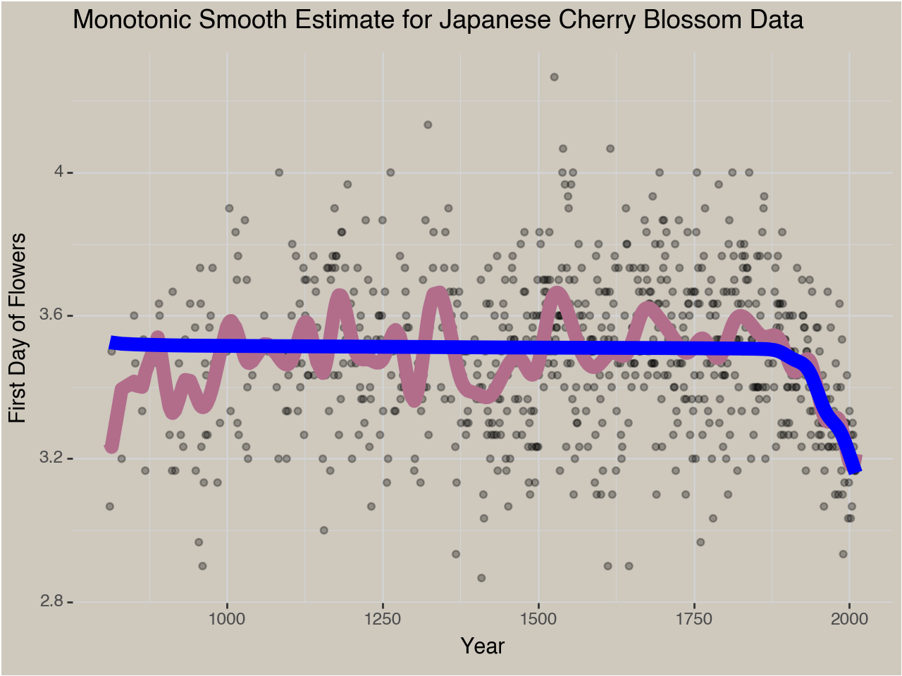
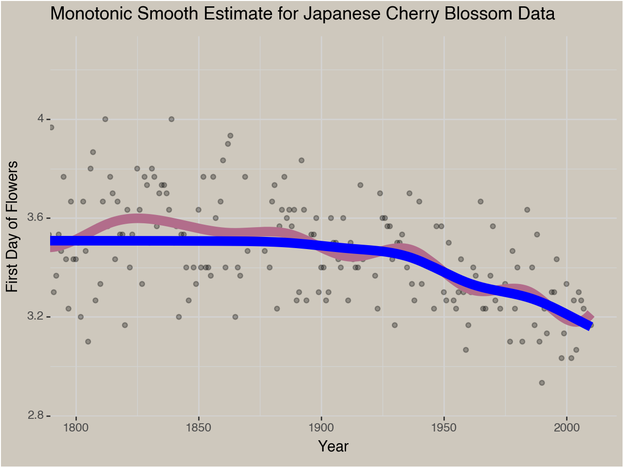
We can zoom in on the parts of the trend that actually decrease to see the difference in the relevant time period more clearly.
Conclussion
The core insight from this post is that we can enforce shape constraints on our functions using a special parameterization of a traditional Generalized Additive Model. You can enforce any number of shapes using slightly different shape matrices. We then used JAX and Scipy to find optimal coefficients for this type of Shape Constrained Additive Model.