In this post I’ll walk through how you can use the same principles behind Gradient Boosting Machines (GBM) to predict parameters of models in the same way traditional GBMs predict 1-dimensional targets. This allows us to get the benefits of Gradient Boosting (large feature sets, high dimensional interactions, modeling at scale) to fit things like smoothing splines, survival analysis, and probabilistic models.
It’s not a modeling silver bullet, but I think this approach can be a useful tool to add to your modeling toolkit. Plus walking through this helped me understand gradient boosting at a deeper level than I did before, so hopefully you feel the same.
Gradient Boosting
Gradient Boosting is a Machine Learning algorithm that fits a series of decision trees; each successive tree attempts to improve the predictions from the set of previous trees. It (generally, there are many GBM implementations out there now) does this with two steps:
- Before fitting a new tree calculate the gradient of the loss function we are minimizing at each observation.
- Fit a new decision tree that predicts the gradient and then add this prediction to the previous predictions.
(*) technically fit the negative gradient, we want the loss to go down
Recently I was reading about Generalized Random Forests (GRF) to learn how they used Random Forests to fit more complicated models than just regression and classification. This post started as a walkthrough of that technique, but I ended up trying something I’ve always had an idea for first; can we use a GBM to fit distributions, not just make individual predictions? To test this I am going to walk through using Gradient Boosting to learn the coefficients for a spline function.
The Data
I’ve downloaded 4 years of the Citi Bike usage data and aggregated by
the number of rides in each hour of each day. I’ve also added the
high and low temperature for that day as well as the inches of rain. If
this were a proper forecasting model you’d want the predicted weather
for a day so your model was properly calibrated, but this is fine for
having features to learn parameters from. One unique thing about this
data is that I have stored the hourly ride counts and the hour of the
day in an aggregated polars array. This is so the splits will work on
the daily level, since I need to generate spline coefficients for each
day and apply them to the 24-hour range. If I was using a traditional
GBM I would use the ride_hour as a feature and predict the hourly
counts.
| dow | woy | year | high_temp | low_temp | precip | ride_date | ride_hour | ride_count |
|---|---|---|---|---|---|---|---|---|
| i8 | i8 | i32 | f64 | f64 | f64 | date | array[i64, 24] | array[u32, 24] |
| 5 | 38 | 2022 | 51.98 | 64.04 | 0.0 | 2022-09-23 | [0, 1, … 23] | [1458, 782, … 2465] |
| 1 | 3 | 2023 | 30.2 | 48.02 | 0.0 | 2023-01-16 | [0, 1, … 23] | [564, 318, … 827] |
| 4 | 34 | 2024 | 62.06 | 77.0 | 0.0 | 2024-08-22 | [0, 1, … 23] | [1840, 999, … 4037] |
| 5 | 26 | 2025 | 64.04 | 73.94 | 0.0787402 | 2025-06-27 | [0, 1, … 23] | [2791, 1683, … 5395] |
| 3 | 34 | 2024 | 59.0 | 75.02 | 0.0 | 2024-08-21 | [0, 1, … 23] | [1744, 903, … 3445] |
Let’s use this data to fit a traditional GBM on the hourly data and visualize some results.
hourly_df = hourly_df.join(zero_days_df, how='anti', on='ride_date')

X_hourly = hourly_df[FEATURE_COLS + ['ride_hour']].to_numpy()
y_hourly = hourly_df['ride_count'].to_numpy()
y_hourly_log = np.log1p(y_hourly)

hourly_gbm = GradientBoostingRegressor(min_samples_leaf=4, validation_fraction=0.05)
hourly_gbm.fit(X_hourly, y_hourly_log)
GBM Regression Feature Importances:
ride_hour: 77.99%
low_temp: 6.20%
high_temp: 4.57%
dow: 3.46%
precip: 2.98%
year: 2.65%
woy: 2.15%
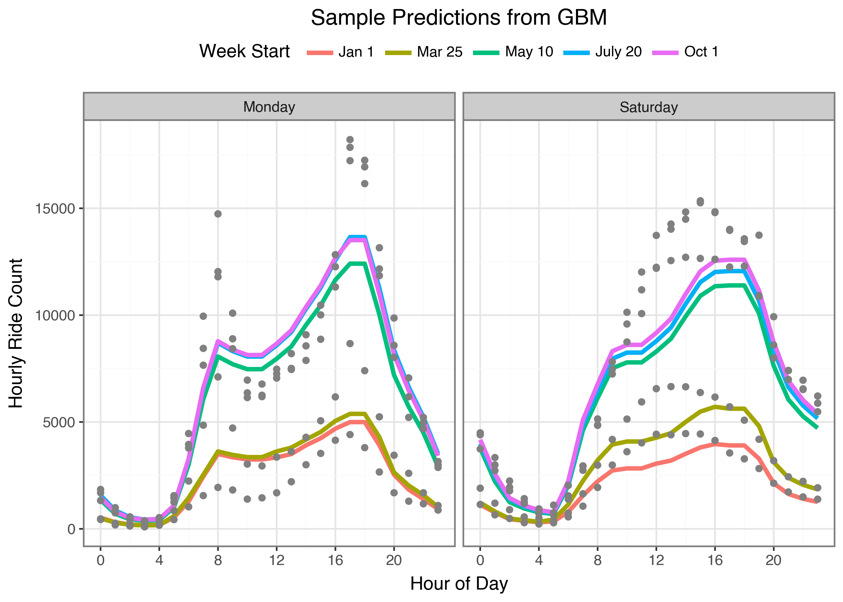
We can see this model has a hard time picking up on the different shapes between weekdays and weekends. It also has some sharp corners that maybe we should try and smooth out. But what if we could use the same process of identifying optimal splits for a single hour’s prediction in order to learn an entire coefficient vector? And yes, I’m just going to get ahead of any comments now; I’m not trying to make either model “the best” I’m only trying to work through the model fitting process. We are here for the journey, not the final validation loss value, ok?
Gradient Boosting as Optimization
Traditionally Gradient Boosting Models are fit by learning the direction to move each prediction individually at each iteration. By calculating the loss value for each observation, and then using the gradient of that observation’s prediction as a “pseudo-label” we can learn a model to make predictions at that step. We can use the same procedure to fit a set of parameters and optimize them with the same algorithm. Then when we need to make a prediction we can use the predicted parameter values for that observation.
In our example we will calculate our parameter vectors $\theta$ for an observation $x$ at any iteration $m-1$ as the sum of all the individual predictions from our base learners $f_m(x)$
\[ \hat{\theta}_{m-1} = \sum_{i \in m-1} f_{m-1}(x) \]The base learners are models learned to predict the gradients of these parameters against our loss function
\[ f_m(x) \sim \nabla L(y, \hat{\theta}_{m-1}) \]In our example we need one extra step. If $b(\theta, x)$ is an individual model that generates predictions for a set of parameters $\theta$ and an observation $x$ then we calculate the gradients by how well the predictions from $b(\theta, x)$ predict our loss function $L$:
\[ \nabla L(y_i, b(\theta_{m-1}, x_i)) \]Then our decision tree will use $-g_{\theta}$ as the multi-target outputs and we can fit a decision tree to these targets. Since we have multiple parameter values in a smoothing spline we use a multitarget algorithm to make predictions for each dimension.
And our updates to our fitted parameters are
\[ \hat{\theta}_{m} = \hat{\theta}_{m-1} + \alpha \cdot f_m(x) \]Let’s ease into this by mimicking what the tree splitting algorithm does to find optimal splits but with our parameters; coefficients for a smoothing spline of the hours of the day.
Optimal Spline Splits
Let’s walk through this without worrying about trees and gradients. The goal here is to pick up on which feature value results in the most unique daily ride shape. We’ll loop through the unique values in a feature as the tree splitting algorithm will do. But for a first pass we will just measure how much variance there is from using the group average to predict the hourly ride counts. So for example we will measure the squared error from the observed counts with a single day of the week’s average, and then do the same for all the other days as one group. The day with the lowest combined Sum of Squared Errors does the best job of splitting the data into coherent days of the week.
shape: (7, 2)
  Day of Week   SSE
  ------------- -----------
  i64           f64
  1             2.1539e11
  2             2.1197e11
  3             2.1273e11
  4             2.1379e11
  5             2.1624e11
  6             2.0468e11
  7             2.0292e11
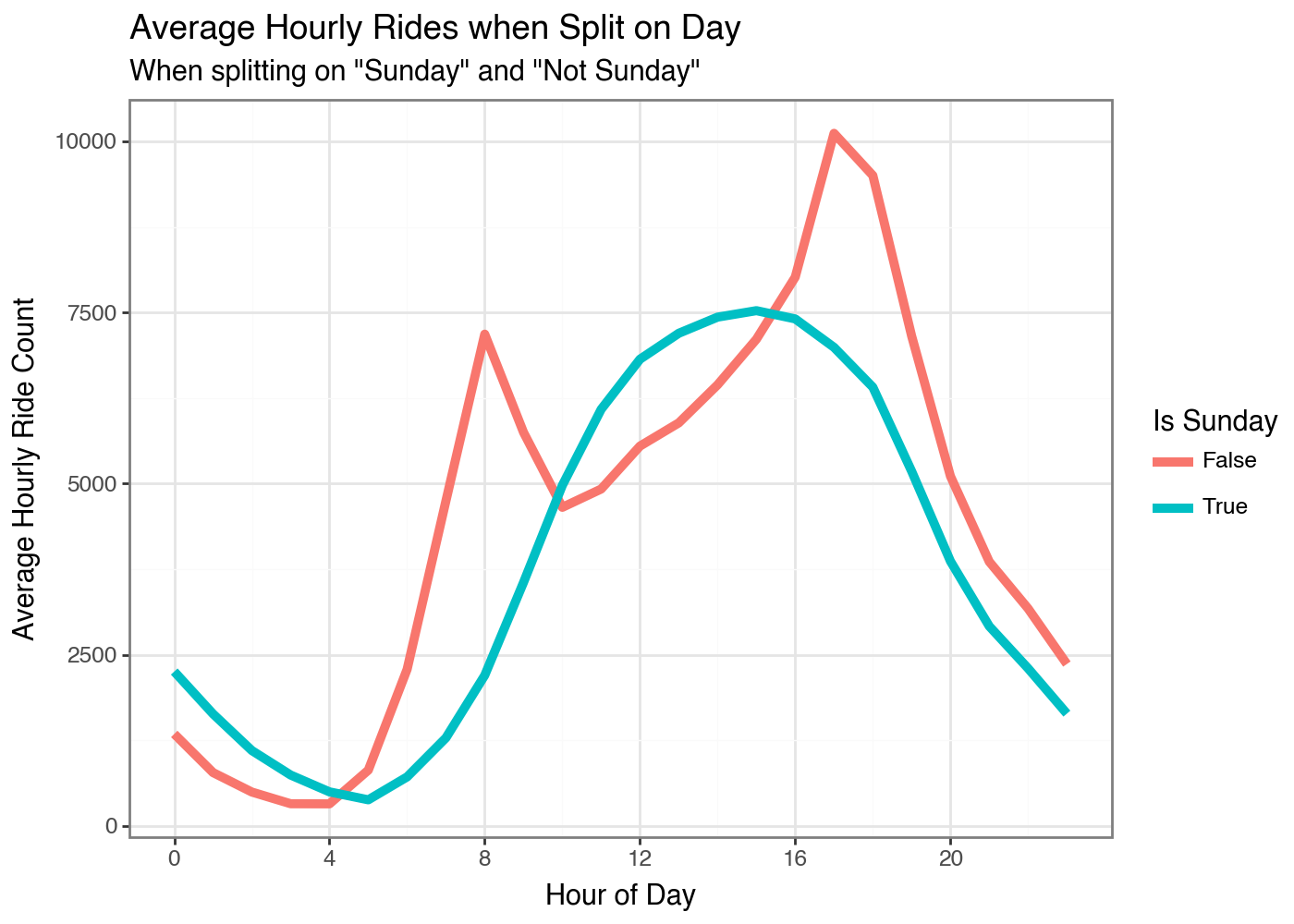
So Sunday has the most unique shape by this measure. The other days would have had more total error across all observations if we had split on one of them instead. We can do the same thing by the Weeks of the Year.
shape: (5, 2)
  Week of Year   SSE
  -------------- -----------
  i64            f64
  14             1.7068e11
  15             1.7146e11
  13             1.7213e11
  12             1.7354e11
  16             1.7379e11
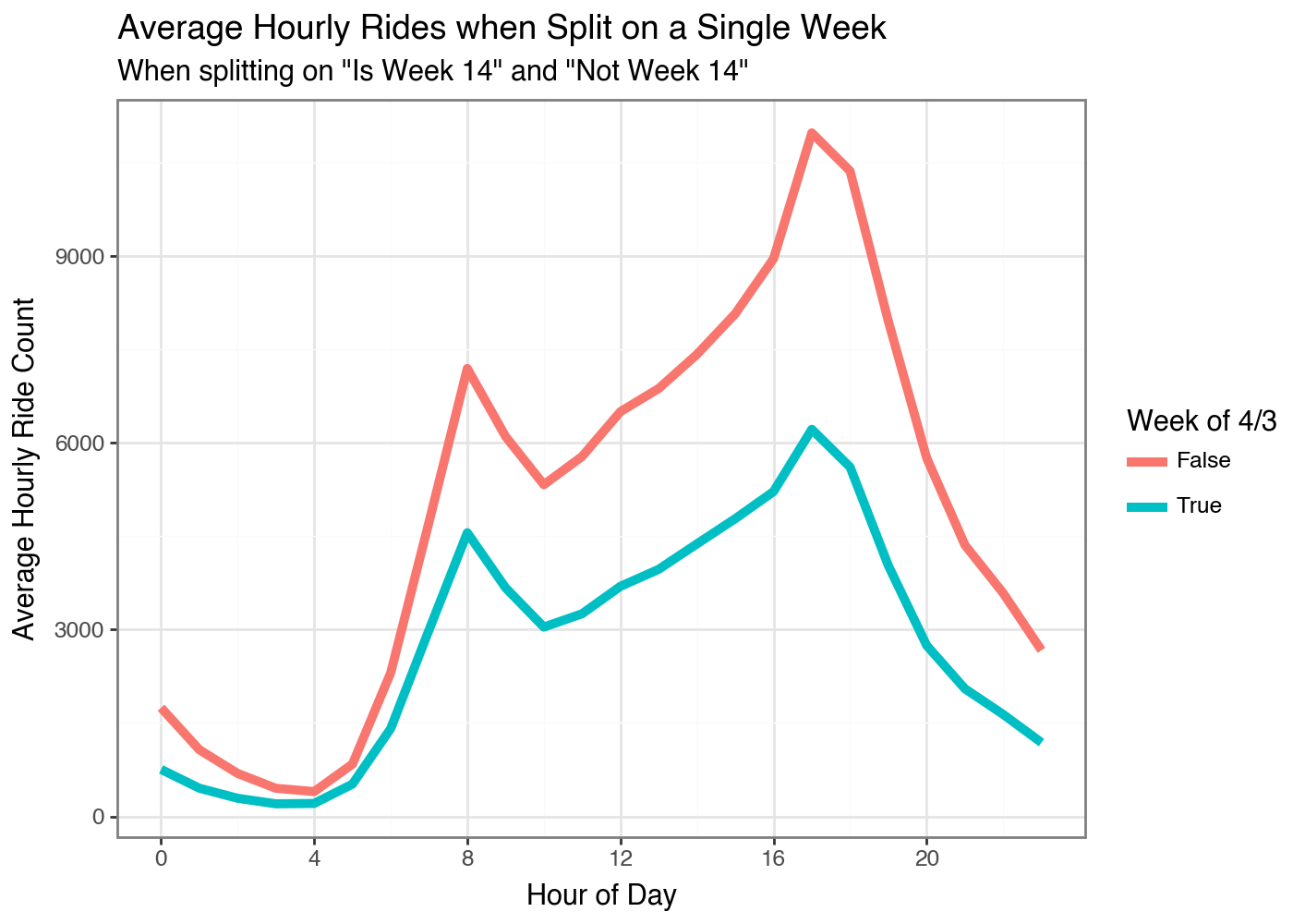
I think this may be a data problem with some values missing or something. I don’t know why early April would have the least amount of rides? Maybe spring break for the kids? Oh wow, that is the answer haha.
Smoothing Splines
Now we can actually get to fitting our Gradient Boosting Spline Model. If you want an introduction to splines I’ve written a couple different posts on this topic:
- How to Fit Monotonic Smooths in JAX using Shape Constrained P-Splines
- A first Look at some Atlanta Housing Data
- Fitting Multiple Spline Terms in Python using GLUM
For our model we have to do a little preprocessing to be ready for the fitting process
- Build our spline basis for the 24 hour period of day
- Write a function to generate predictions with our flattened hourly data
- Write a function to calculate the gradient of our loss function
N_KNOTS = 12
x_day = hourly_df['ride_hour'].unique().to_numpy().reshape(-1, 1)
spline_hour = SplineTransformer(n_knots=N_KNOTS, include_bias=True).fit(X=x_day)
N_SPLINES = spline_hour.n_features_out_

bs_day = spline_hour.transform(x_day)
print('Example of Basis Activations for different hours')
for i in range(6):
    print(f'Hour {i*4}: {display_vec(bs_day[i*4, :])}')
Example of Basis Activations for different hours
Hour 0: ▂█▂▁▁▁▁▁▁▁▁▁▁▁
Hour 4: ▁▁▃█▂▁▁▁▁▁▁▁▁▁
Hour 8: ▁▁▁▁▃█▂▁▁▁▁▁▁▁
Hour 12: ▁▁▁▁▁▁▄█▁▁▁▁▁▁
Hour 16: ▁▁▁▁▁▁▁▁▅█▁▁▁▁
Hour 20: ▁▁▁▁▁▁▁▁▁▁▆█▁▁
Here is where things start to diverge from traditional models though. I
do not want each tree $f_m(x)$ to produce a prediction of $\hat{y}_m$. I
want each tree to predict the optimal spline coefficients for that
gradient step $\hat{\theta}_t$. So we will need to know the gradient of
the loss function for each spline coefficient and each observation.
Luckily, jax makes this easy. We can define our loss function once
that operates on a single observation. Jax will then calculate the
partial derivatives automatically with grad. And we can scale this to an
array with the vmap function.
def loss_i(coefs, bs_array, y_array):
    """
    Calculate the scalar loss for the input, spline transformed data

    Parameters:
    coefs: [b,] 1d array from numerical procedure
    bs_array: [24, b] spline transformed data
    y_array: [24, 1] target values
    """
    #x_array_ = x_array.reshape(-1, 1)
    y_array_ = y_array.reshape(-1, 1)

    preds = jnp.dot(bs_array, coefs.reshape(-1, 1))
    error = jnp.power(preds - y_array_, 2)
    penalty = jnp.sum(jnp.square(jnp.diff(coefs, 1)))
    # using mean instead of sum to keep the total loss numbers low...I think that's ok
    error_array = jnp.mean(error)
    return error_array + 0.01 * penalty

# vectorize our loss function to work on arrays
loss_array = vmap(loss_i)
# Calculate the gradient of a single observation
# grad only works on scalar output, so we have to vectorize them separately
grad_i = grad(loss_i)
grad_array = vmap(grad_i)

v, g = value_and_grad(loss_i)(coefs_init, BS_daily[0], y_log[0])
print(f'Loss function value for one day: {v:.2f}')
print('Gradients for each spline coefficient for that day:')
print(np.round(g, 2))
Loss function value for one day: 1.28
Gradients for each spline coefficient for that day:
[ 0.01        0.11        0.29        0.28        0.         -0.14
 -0.13       -0.16       -0.19999999 -0.22999999 -0.17       -0.06
 -0.          0.        ]
I’ve initialized some coefficients to predict a flat line, coefs_init.
We can calculate our initial gradients and thus pseudo-labels to use in
the first tree with our gradient functions. One technical note is the
coefficient vector needs to be the same length as the X and Y arrays I’m
using for vmap to accept it. Once we start fitting trees this will be
the case, but when I created my coefs_init values originally I just used
a 1d array for all values. That’s why in the following code cell I
repeat it to match the length of our data.
coefs_init_array = np.tile(coefs_init, (daily_df.shape[0], 1))
labels_init = -grad_array(coefs_init_array, BS_daily, y_log)
print(labels_init.shape)
(1432, 14)
Gradient Boosting Splines
We now have everything we need to update our spline coefficients:
coefs_init: an initial set of smoothing splines to produce a flat predictiongrad_array: a function to calculate the gradients of our predictions with respect to the coefficients at each observationlabels_init: The initial gradient values to use as a our pseudo-labels for our first iteration
Let’s fit one decision tree with our features to predict the gradients of the splines for each observation
from sklearn.tree import DecisionTreeRegressor
x_features = daily_df[FEATURE_COLS].to_numpy()
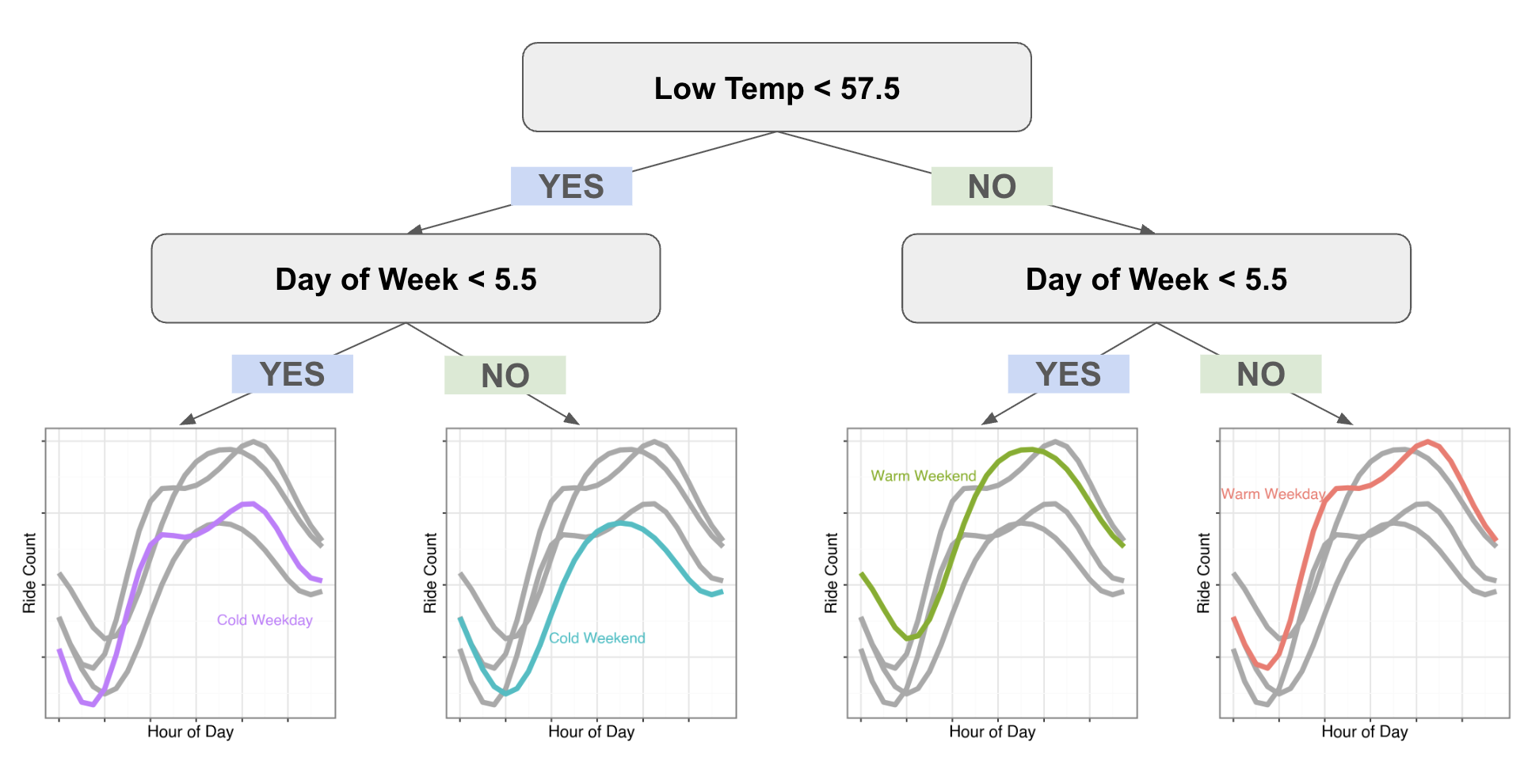
tree_init = DecisionTreeRegressor(max_depth=2).fit(x_features, labels_init)
Tree splits:
low_temp <= 57.5
  dow <= 5.5
  else:
else:
  dow <= 5.5
  else:

First Tree Feature Importances:
low_temp: 64.93%
dow: 35.07%
woy: 0.00%
year: 0.00%
high_temp: 0.00%
precip: 0.00%
We can see how the different predictions look for this leaf nodes of this simple tree:
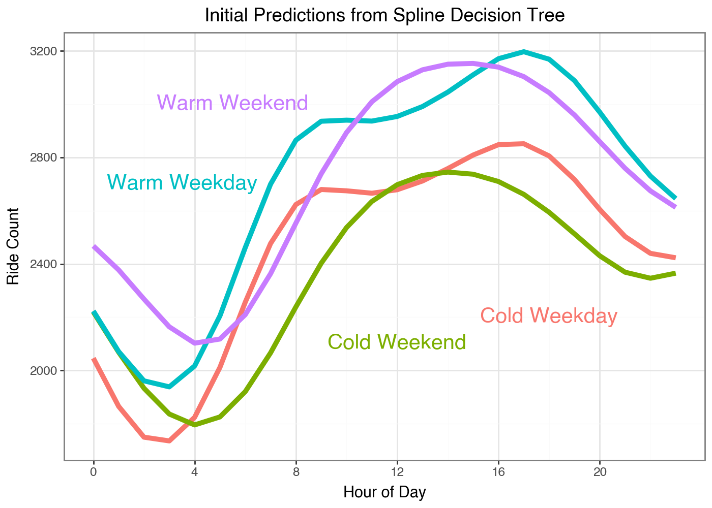
What I love is we can immediately see the different shapes in the weekends and weekdays. Our classic GBM had to learn the trend at each hour of the day so it took a while until the differences in curves were the largest residual signal left to optimize against. But with our Gradient Boosted Splines our model can learn the full curve in one go.
I also want to point out I’m not clustering the data and then fitting a model to each subset of data to learn the coefficients. These predictions are only coming from predicting the gradients of the loss function on each day from a flat line. The model learns the optimal splits to cluster the data on for optimizing our loss function. We’ve basically created a supervised clustering algorithm.
Gradient Boosted Splines
We now have everything we need to fit our Gradient Boosting models to try and improve our predictions.
def fit_tree_and_update(
        coefs,
        bs_array=BS_daily,
        y_array=y_log,
        x_features=x_features,
        lr=0.1):
    """Fit a single tree and update the predictions"""
    # 1. Calculate Gradients
    labels = grad_array(coefs, bs_array, y_array)
    # 2. Fit a tree
    tree = DecisionTreeRegressor(max_depth=2).fit(x_features, labels)
    # 3. Get predictions of the spline coefficients
    tree_preds = tree.predict(x_features)
    # 4. Update our model fits
    new_coefs = coefs - lr * tree_preds
    return new_coefs, tree, tree_preds

N_TREES = 500

preds_init = predict_array(coefs_init_array, BS_daily).squeeze(1)
loss_init = loss_array(coefs_init_array, BS_daily, y_log).mean()

tree_params = coefs_init_array
spline_trees = []
for i in range(N_TREES):
    result = fit_tree_and_update(tree_params, BS_daily, y_log, x_features)
    tree_params = result[0]
    spline_trees.append(result)

# get the last tree's predictions
coef_fit = spline_trees[-1][0]
preds_fit = predict_array(coef_fit, BS_daily).squeeze(1)
loss_fit = loss_array(coef_fit, BS_daily, y_log).mean()

print(f'Initial loss: {loss_init}')
print(f'Final loss: {loss_fit}')
Initial loss: 1.5850720405578613
Final loss: 0.2547142207622528
So the model (spline_trees) predicts a coefficient vector for each
observation. To get predictions for each hour at each observation (an
observation is a single day’s hourly totals) we need to apply each
coefficient vector against the Spline Basis we created for the 24 hour
period initially. predict_array is a function I wrote to generate the
actual hourly predictions based off a customized coefficient vector.
[6.8599997 6.47      6.1099997 5.95      6.12      6.67      7.3999996
 8.0199995 8.42      8.57      8.559999  8.55      8.599999  8.69
 8.79      8.9       8.99      9.01      8.92      8.73      8.48
 8.21      7.98      7.8199997]
[7.29 6.66 6.08 5.59 5.62 6.67 7.82 8.59 8.9  8.67 8.48 8.55 8.7  8.81
 8.95 9.05 9.15 9.3  9.17 8.83 8.38 8.04 7.9  7.81]
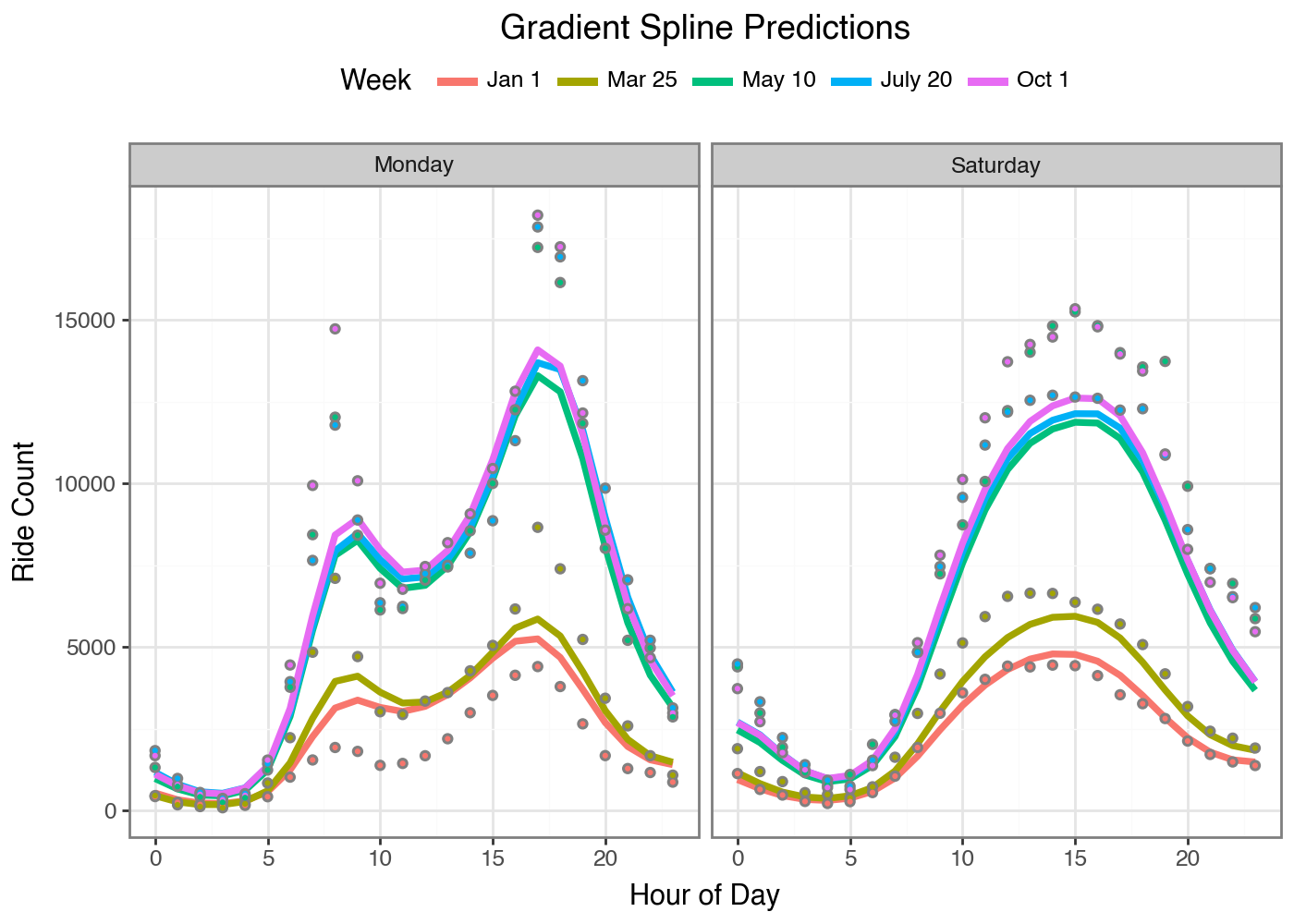
Let’s compare our fitted Gradient Boosted Spline to our initial GBM. The
model is still undershooting the peaks and misses something about the
January 1st day (I should probably add a Is_Holiday feature). But we
get smooth curves! From Gradient Boosting! It’s amazing that this
approach can be accomplished so easily with code by leveraging open
source tools like Jax and Scikit-Learn. All you need is a loss function
and a way to express individual predictions from a set of parameters and
you can fit any model this way.
I’m sure there are tons of valid inference questions you could ask of this approach; I don’t have those answers. But I think that will be it for today’s post. I’m excited to take this concept even further to fit more types of models. If you want to make sure you see any future posts I write you can follow me @statmills on Twitter or BlueSky. If you are interested in the code for this blog post I’ve added everything to my GitHub repo.
Humanity Oath: I solemnly swear that I did not use AI to write the words in this piece.