Recently I encountered an interesting paper from the facebook research team that outlines a method for using decision trees (specifically boosted trees) to create transformed data to be used as input to a final logistic regression. I thought this was really cool and wanted to try and recreate the method in R. I’ll let the paper authors explain the process for how they went about this.
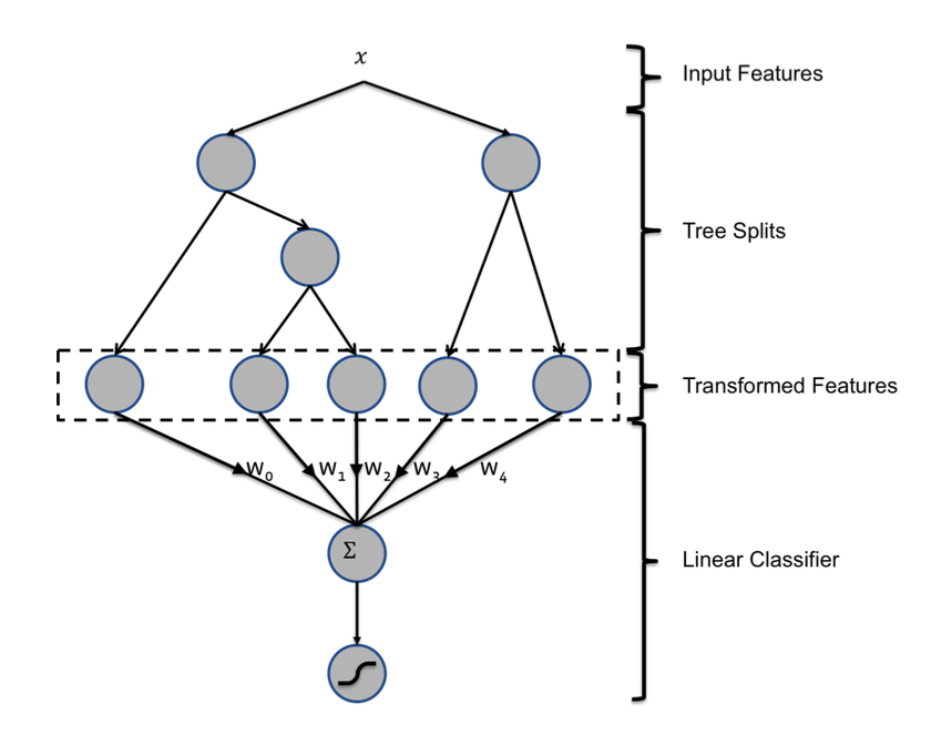
We treat each individual tree as a categorical feature that takes as value the index of the leaf an instance ends up falling in. We use 1-of-K coding of this type of features. For example, consider the boosted tree model in Figure 1 with 2 subtrees, where the first subtree has 3 leafs and the second 2 leafs. If an instance ends up in leaf 2 in the first subtree and leaf 1 in second subtree, the overall input to the linear classifier will be the binary vector [0, 1, 0, 1, 0], where the first 3 entries correspond to the leaves of the first subtree and last 2 to those of the second subtree.
Essentially each tree represents a dummy variable and the terminal node that each observation ends up in represents a different level of that variable. Here is a picture from the paper diagramming the process:
I’m by no means an expert on using decision rules as input to regression models but I have not heard of this exact way to transform raw data to use as input to a different model but if there has been other research on this topic please feel free to share, I’d love to read more about it.
Their paper shows that this method was more accurate than either the Gradient Boosting Machine (GBM) or the Logistic Regression alone but they didn’t go into any detail on how they traversed the tree so I’ll try to focus on that since it was not the easiest thing to code up. I’ll be using the Lending Club Loan Data found on Kaggle as my test set for no other reason than it has many samples and many different features. It’s actually a little too big, the steps in this script do take a while so if you want to recreate the results you’ve been warned. I’ll be doing some small data cleansing which you can see in the source code for this post but I won’t be showing it here to save space. The dataset is a mix of categorical and numeric values so this should be a good use case for using the trees to find relationships between the underlying variables and the loan status. I assume, and hope to test, if the data was just numeric variables then the trees wouldn’t improve much over just using smoothing splines.
Modeling Strategy
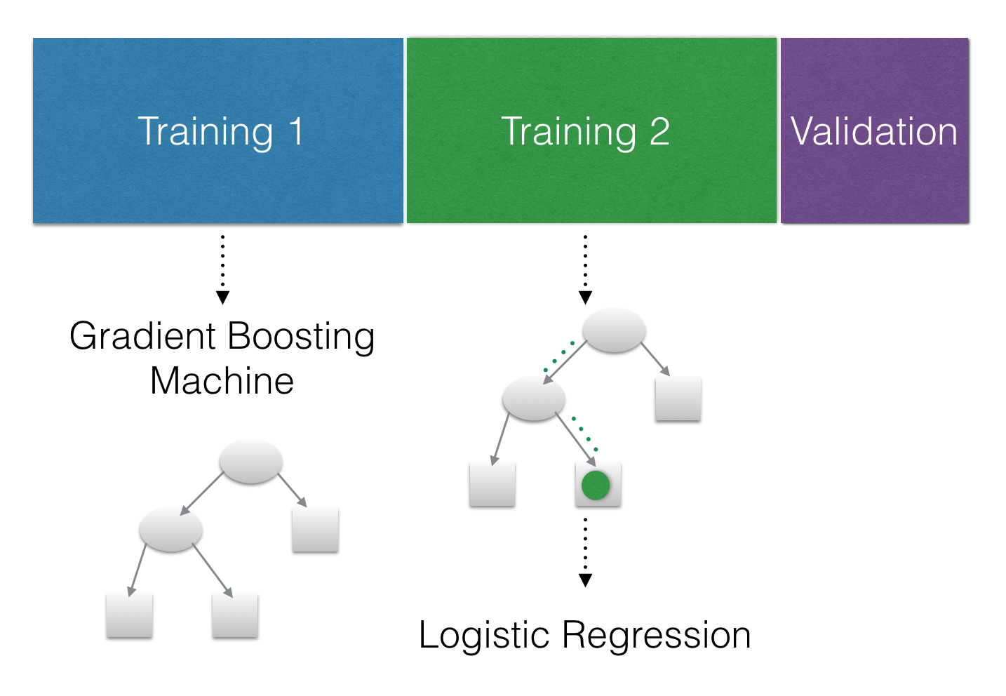
Although the paper showed that this method was more accurate on their data I’d still like to test its accuracy in comparison to other methods. To do this we need to plan our modeling strategy. We have two models to fit to the data; A GBM to transform the raw data to the leaf positions and a Logistic Regression on the transformed data. We should use different datasets to train these two models so that we don’t overfit the Logistic Regression. We will also need a third validation dataset to test the accuracy on data that the models haven’t seen so we have an unbiased estimate of how well the models perform. I’m going to do a 40-40-20 split on the loan data. Here is a totally sweet diagram to show what I mean:
Train a Gradient Boosting Model
Let’s get started training the GBM. While using the xgboost or h2o package
would be faster than the gbm package I am more familiar with the output of
the gbm function and know that it contains the tree and split information
we need. Traversing each tree to find the leaf positions took a lot of thought
and trial and error so I figured the time I saved on tuning the model wouldn’t
make up for the extra time it took me to code it up.
set.seed(21091)
set_id <- sample(c(1, 2, 3), size = nrow(clean_data), replace = T, prob = c(.4, .4, .2))

training_data_1 <- clean_data[set_id == 1, ]
training_data_2 <- clean_data[set_id == 2, ]
validation_data <- clean_data[set_id == 3, ]

gbm_model <- gbm(formula = bad_loan ~ .,
                data = training_data_1,
                interaction.depth = 2,
                distribution = "bernoulli",
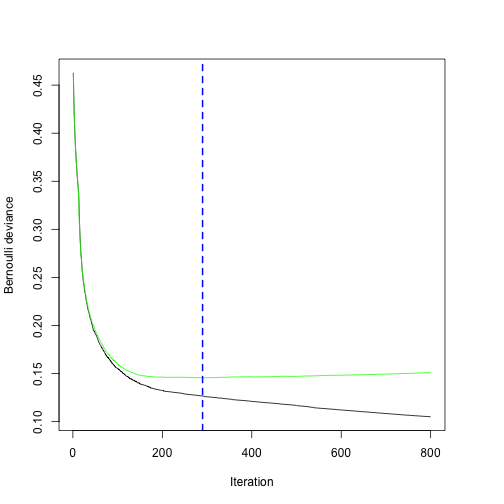
                cv.folds = 5,
                shrinkage = .1,
                n.trees = 800)
# Refit the model to the appropriate number of trees
gbm_model <- gbm(formula = bad_loan ~ .,
                 data = training_data_1,
                 interaction.depth = 2,
                 distribution = "bernoulli",
                 shrinkage = .1,
                 n.trees = 290,
                 keep.data = F)
Traverse the Trees
Now that we have the fitted model we need to send the second training set
through the GBM to find the leaf positions of each observation. To do this I
wrote a helper function called traverse_trees. It may be tough to follow
along but here is the basic structure:
- For each tree find the split decisions
- For each split decision generate a logical index of the underlying data for the left and right path
- Combine any multi-layer splits.
- Use the logical indexes to generate the dummy variables for each terminal node
There are certainly ways to make this function better. I rely on the depth of the GBM to always be two so I don’t do any recursive partitioning to make it more robust. It’s all embarrassingly parallel so could easily be made faster. But for a quick exploratory analysis I’m cool with it.
traverse_trees <- function(boosted_model, predict_data){

  n_trees <- boosted_model$n.trees
  category_splits <- boosted_model$c.splits
  col_types <- vapply(predict_data, class, character(1))
  matrix_stuff <- c()

  for(i in seq_len(n_trees)){
    #extract the tree
    tree <- pretty.gbm.tree(boosted_model, i.tree = i)

    # add one to each var (the gbm.object is 0 indexed, gross)
    tree$SplitVar <- tree$SplitVar + 1

    # Get info about the non-terminal nodes into a list
    split_info <- tree %>%
      mutate(node = row.names(.)) %>%
      filter(SplitVar != 0) %>%
      apply(1, function(x) {
      temp_list <- list(node = unname(x["node"]),
                        split_var = as.numeric(unname(x["SplitVar"])),
                        split_num = as.numeric(unname(x["SplitCodePred"])),
                        left_child = unname(x["LeftNode"]),
                        right_child = unname(x["RightNode"]),
                        missing_child = unname(x["MissingNode"]))
      return(temp_list)
    })

    # function to get logical indicators for the observations at each split
    traverse <- function(tree_info, category_splits, obs_data, col_types){

      split_var <- names(obs_data)[tree_info$split_var]
      # check for missing values in the data
      missing_flag <- any(is.na(obs_data[[split_var]]))

      if(col_types[tree_info$split_var] == "factor") {
        # find the direction the tree puts each value
        level_directions <- category_splits[[tree_info$split_num + 1]]
        var_levels <- levels(obs_data[[split_var]])
        # assign the levels to the left and right splits
        left_levels <- var_levels[level_directions == -1]
        right_levels <- var_levels[level_directions == 1]
        # turn each into a list
        left_list <- list(lgl = obs_data[[split_var]] %in% left_levels,
                          parent = tree_info$node)
        right_list <- list(lgl = obs_data[[split_var]] %in% right_levels,
                           parent = tree_info$node)
      } else {
        # I actually don't know if it's <= & > or < & >=
        left_list <- list(lgl = obs_data[[split_var]] <= tree_info$split_num,
                          parent = tree_info$node)
        right_list <- list(lgl = obs_data[[split_var]] > tree_info$split_num,
                          parent = tree_info$node)
      }

      # if the tree uses missing values then just add on an extra list
      if(missing_flag) {
        miss_list <- list(lgl = is.na(obs_data[[split_var]]),
                          parent = tree_info$node)
        split_list <- list(left_list, right_list, miss_list)
        names(split_list) <- c(tree_info$left_child, tree_info$right_child, tree_info$missing_child)
      } else {
        split_list <- list(left_list, right_list)
        names(split_list) <- c(tree_info$left_child, tree_info$right_child)
      }

      return(split_list)
    }

    # for each split node find the children
    terminal_info <- map(split_info, traverse, category_splits = category_splits, obs_data = predict_data, col_types = col_types) %>% flatten

    terminal_nodes <- row.names(tree)[tree$SplitVar == 0]
    splits <- names(terminal_info)
    # for each terminal node find out if it has a parent
    # if so then include the parent logical vector
    full <- map_if(terminal_info, ~ .x$parent %in% splits, function(x, tree_info) {
      x[["lgl"]] <- x[["lgl"]] & tree_info[[x$parent]][["lgl"]]
      return(x)
    }, terminal_info)

    output <- full[terminal_nodes] %>% # only keep the terminal nodes
      # if there are no missing values then remove that terminal node
      discard(~is.null(.x)) %>%
      map(extract2, "lgl") %>%
      unlist

    obs <- matrix(output * 1, nrow = nrow(predict_data), byrow = F)
    stopifnot(all(rowSums(obs) == 1))
    matrix_stuff <- cbind(matrix_stuff, obs)
  }

  return(matrix_stuff)
}

tree_output <- traverse_trees(gbm_model, training_data_2)
To recap what we just did here is how this process works for the first tree.
We can use the pretty.gbm.tree function from the gbm package to view the
splits in the first tree:
| SplitVar | SplitCodePred | LeftNode | RightNode | MissingNode | ErrorReduction | Weight | Prediction | |
|---|---|---|---|---|---|---|---|---|
| 0 | 36 | 1.8000000 | 1 | 5 | 6 | 4268.57 | 177368 | -0.0004912 |
| 1 | 38 | 0.0000000 | 2 | 3 | 4 | 614.49 | 172512 | -0.0376891 |
| 2 | -1 | -0.0680307 | -1 | -1 | -1 | 0.00 | 149788 | -0.0680307 |
| 3 | -1 | 0.2032145 | -1 | -1 | -1 | 0.00 | 19216 | 0.2032145 |
| 4 | -1 | -0.0617460 | -1 | -1 | -1 | 0.00 | 3508 | -0.0617460 |
| 5 | -1 | 1.3209838 | -1 | -1 | -1 | 0.00 | 4856 | 1.3209838 |
| 6 | -1 | -0.0004912 | -1 | -1 | -1 | 0.00 | 177368 | -0.0004912 |
The tree is 0 indexed so we want to look at the 37th and 39th variable in our data:
| bad_loan | recoveries | last_pymnt_d |
|---|---|---|
| 0 | 0.00 | Jun-2014 |
| 0 | 0.00 | Jan-2016 |
| 1 | 269.29 | Nov-2012 |
| 0 | 0.00 | Jan-2015 |
| 0 | 0.00 | Jan-2015 |
This tree uses the recoveries variable to make its first split and for
small amounts of that (less than 1.8) it checks the month of last_pymnt_d.
There are some missing observations in that variable so we have 4 nodes for
this tree
##      [,1] [,2] [,3] [,4]
## [1,]    1    0    0    0
## [2,]    1    0    0    0
## [3,]    0    0    0    1
## [4,]    1    0    0    0
## [5,]    1    0    0    0
Train a Logistic Regression Model
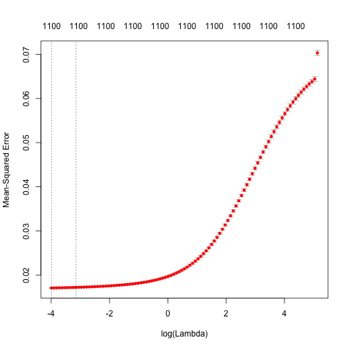
Now we can get on to our logistic regression. I’ll use the cv.glmnet
function from the glmnet package to fit a Penalized Logistic
Regression using 5-fold cross validation.
Y <- training_data_2$bad_loan

ridge_regression <- cv.glmnet(x = tree_output, y = Y, nfolds = 5, alpha = 0)
Model Performance
val_output <- traverse_trees(gbm_model, validation_data)

gbm_preds <- predict(gbm_model, newdata = validation_data, type = "response", n.trees = 290)
boosted_logistic_preds <- predict(ridge_regression, newx = val_output, type = "link", s = "lambda.1se")[, 1]
boosted_logistic_preds <- 1 / (1 + exp(-boosted_logistic_preds))

val_response <- validation_data$bad_loan

perf_gbm <- c("MSE" = mean((val_response - gbm_preds)^2), "AUC" = glmnet::auc(val_response, gbm_preds))
perf_boost_ridge <- c("MSE" = mean((val_response - boosted_logistic_preds)^2), "AUC" = glmnet::auc(val_response, boosted_logistic_preds))

rbind(perf_gbm, perf_boost_ridge)
##                         MSE       AUC
## perf_gbm         0.01619194 0.9725718
## perf_boost_ridge 0.24403963 0.9672341
Wow, the GBM alone performs much better by Mean Square Error (MSE) than the boosted tree + ridge regression model. Let’s look at how the models are calibrated.
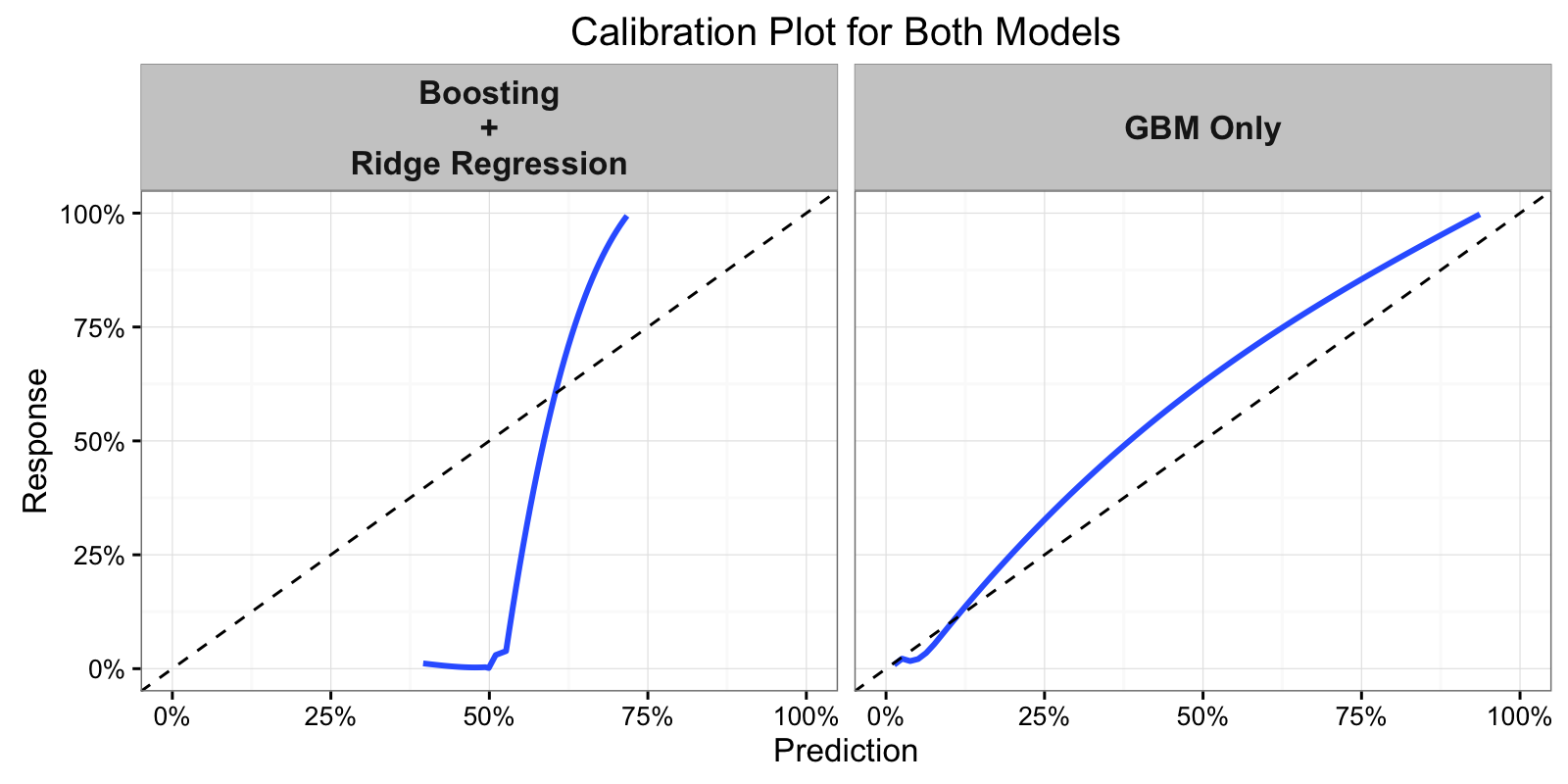
The fact that the boosted + ridge model performed so poorly by MSE but still
has a relatively high AUC implies, at least to me, that the penalized
regression was too restrictive. The model separates the bad from good very
well (as evidenced by a high AUC) but is poorly calibrated. Perhaps if we
used an actual logistic regression and not ridge regression we would see
better results? And I know this is using the validation set to influence your
decisions but I gots to know.
Unfortunately with a dataset of this size (the training output used to fit
the ridge regression was 354852 rows by 1104 columns) R’s base glm won’t
work. We can use the h2o package to fit one though.
h2o is a pretty incredible resource to fit large models
by using distributed computing on a JVM, if you haven’t heard of them I
really encourage you to check out their resources.
library(h2o)
# initialize large local cluster
localH2O <- h2o.init(min_mem_size = "1g", max_mem_size = "4g")
# load the tree output into the h2o environment
logistic_h2o_df <- as.h2o(data.frame(tree_output))
# add the dependent variable
bad_loan <- as.h2o(select(training_data_2, bad_loan) %>% mutate(bad_loan = factor(bad_loan)))
logistic_h2o_df <- h2o.cbind(logistic_h2o_df, bad_loan)
# fit the regression model
logistic_h2o_model <- h2o.glm(x = seq(1, ncol(tree_output)),
                              y = "bad_loan",
                              training_frame = logistic_h2o_df,
                              lambda = 0,
                              family = "binomial")
# get validation data into h2o
logisitc_val_df <- as.h2o(data.frame(val_output))
h2o_preds <- predict(logistic_h2o_model, newdata = logisitc_val_df)
h2o_preds <- as.data.frame(h2o_preds)
##                         MSE       AUC
## perf_gbm         0.01619194 0.9725718
## perf_boost_ridge 0.24403963 0.9672341
## perf_h2o         0.01226116 0.9800423
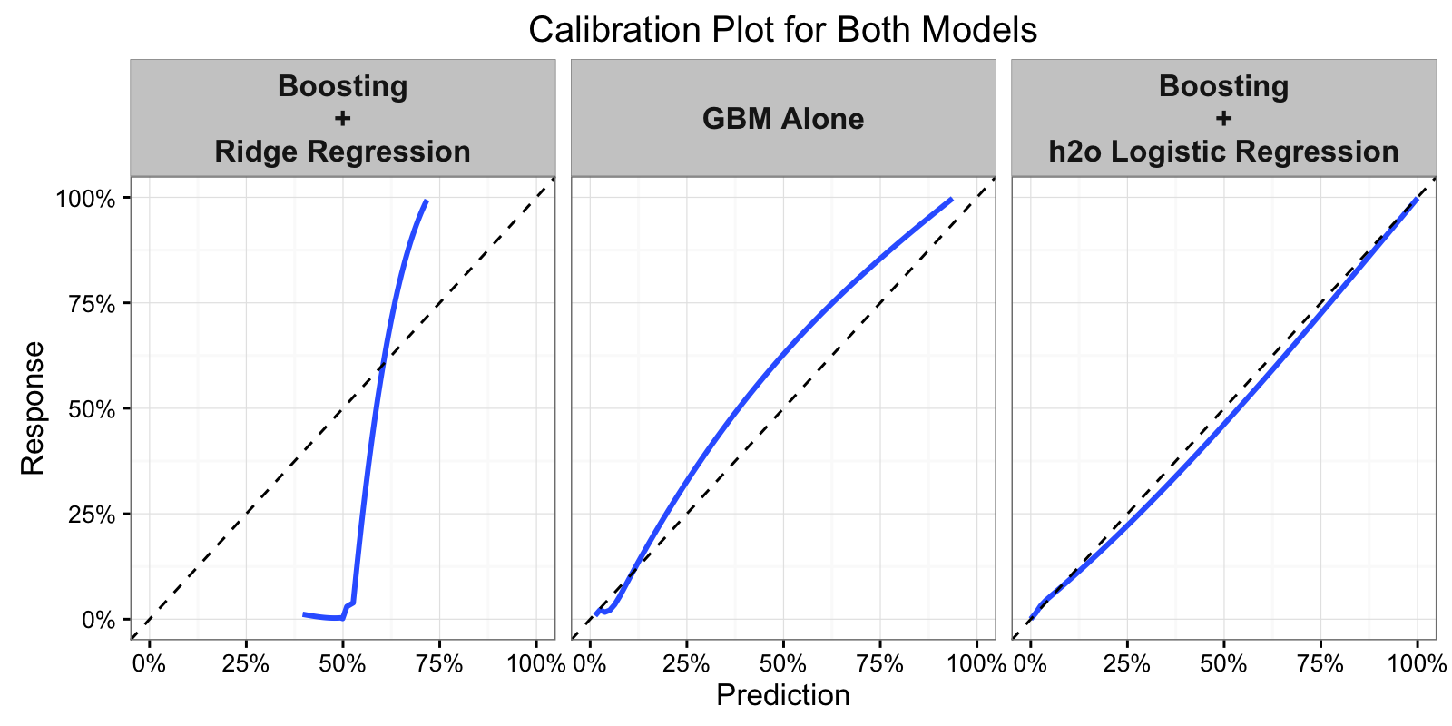
And there it is, using a full Logistic Regression Model we get improved results over the GBM alone by MSE, AUC, and the calibration of the model.
This was a fun exercise for me that allowed me to work out my R muscles and learn a new modeling strategy. I hope you enjoyed it too and if you have any questions or comments please leave a comment or reach out on twitter. As always you can view the source code for this post on github